A Simple CFD Example
In this section, we will study basic visualization techniques for scalar and vector fields by working with a small CFD data set.
The Data
The data that we will work with is the same as used in the COVISE tutorial. It is distributed in the COVISE source repository and comes with every COVISE installation in the subdirectory .../share/covise/example-data/tutorial. You can also get it by downloading the raw contents of the files in this directory from GitHub. It is provided in native COVISE format. It shows the results of a flow simulation in a channel with two inlets and contains scalar data fields for pressure (tiny_p.covise), temperature (tiny_te.covise) and viscosity (tiny_vis.covise) as well as the velocity vector field (tiny_ve.covise) on an unstructured grid (tiny_geo.covise).
Reading the Data
Reading of data in COVISE format is accomplished with the ReadCovise or ReadCoviseDirectory modules. Both can read up to three fields mapped onto the same grid. The first can handle grid and field data at arbitrary locations in the filesystem. The latter requires that grid and field data reside in the same directory – with the advantage of a more comfortable user interface for selecting the fields to be read.
To start, drag ReadCoviseDirectory from the module library to the empty canvas in the center of the graphical user interface. This will start the module and show a representation of it as a turquoise box. Then continue with selecting the directory where to find the data. This is a parameter of the module. Select the module by clicking on the turquoise box. A pink outline indicates that this module is selected. The user interface will show the parameters of this module in the parameter area. Make sure that only this module is selected – otherwise the GUI will not enable the module parameters view.
In the area labeled Parameters: ReadCoviseDirectory find the line for the directory parameter and click on the folder icon.
This will bring up a file browser window.
Use it to navigate to the directory where you have the COVISE source code. From there, continue to share/covise/example-data/tutorial and click on Choose.
The module will search the directory for files with the extension .covise and will present them in the parameter combo boxes (drop down lists) for grid, normals, and the data fields field0, field1, …
At this stage, we are only interested in the geometric structure of the computational domain.
So it is sufficient to select tiny_geo on the grid parameter.
Execute the workflow by double-clicking on the module or by clicking on the gears icon in the toolbar.
Workflow geo-read shows the module with the selected directory and the grid file.
Examining the Geometry
Here we will study techniques to visualize the geometry of the computational domain. This will also help you to provide context for the visualization of the scalar and vector fields.
Find the Extents of the Geometry Domain
The BoundingBox module takes its geometry input and finds global minimum and maximum values for its coordinates. The result of this process can be seen in its parameter window as the values of the min and max parameters. And of course, it can compute a tight axis-aligned cuboid around the domain of the data. This surrounding box can guide you to the interesting areas of space, it can provide visual clues that help with orientation in 3D space.
The numerical values can be used to provide input for modules requiring coordinates as parameter input.
This bounding box can also be inspected visually by loading it into the COVER renderer. This will open up another window. Connect the output of BoundingBox to the input of COVER and rerun the workflow. You can bring the bounding box into view by clicking on the View All icon in the toolbar right of the animation controls in the COVER window. This will show the bounding box in a light gray color. In order to get an idea of the location and size of the bounding box, you can enable a unit sized coordinate system in the renderer by enabling it with the View Options -> Show axis in the menu of the COVER window. The coordinate system will be shown in red, green, and blue colors for the x, y, and z axes, respectively.
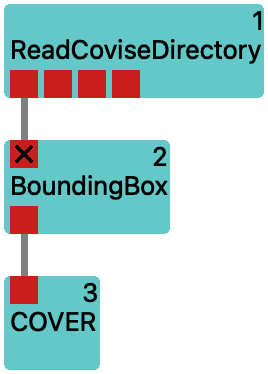
Workflow geo-bounds shows how to compute and display geometry bounding box.
Show the Boundary of the Geometry Domain
The shape of the computational domain can be visualized with the DomainSurface module. It is available from its first, i.e. left-most output. After connecting it to COVER and executing the workflow, it will show the outer surface of the geometry in a light gray color. If you are interested what triangles make up this surface, you can show visualize them by switching to Wireframe in the View options -> Draw style menu of COVER. This will show the outlines of the triangles.
It also provides a second output port providing lines showing the edges of the domain. Currently, this is only a rough approximation, as only those edges that do not neighbor with other cells are shown. Connect also this second output to the input of COVER and execute the workflow again.
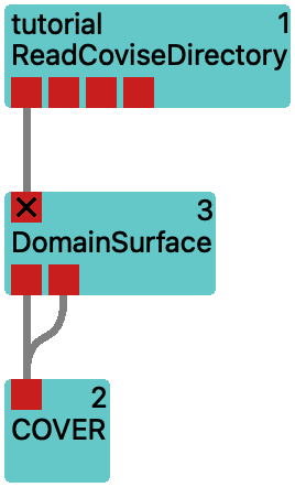

Workflow geo-surface shows how to compute the geometric domain.
Show the Tessellation of the Geometry Domain
Often, the computational domain is discretized by subdividing it into cells. The module ShowGrid can be used to visualize this subdivision. Different to using DomainSurface together with the Wireframe draw style, this will show you what goes on inside the domain.
In order to peek into the domain, it is necessary to disconnect the first output of DomainSurface from the input of COVER. Do so by double-clicking on the line representing this connection. Then connect the output of ShowGrid to the input of COVER and execute the workflow again.
Showing the outline of a large number of cells can be very taxing on the graphics hardware, especially for NVIDIA gaming cards. Restrict the cells to show by selecting only specific types of cells or by supplying a list of cell IDs.
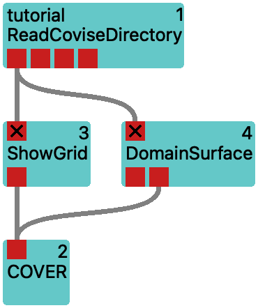
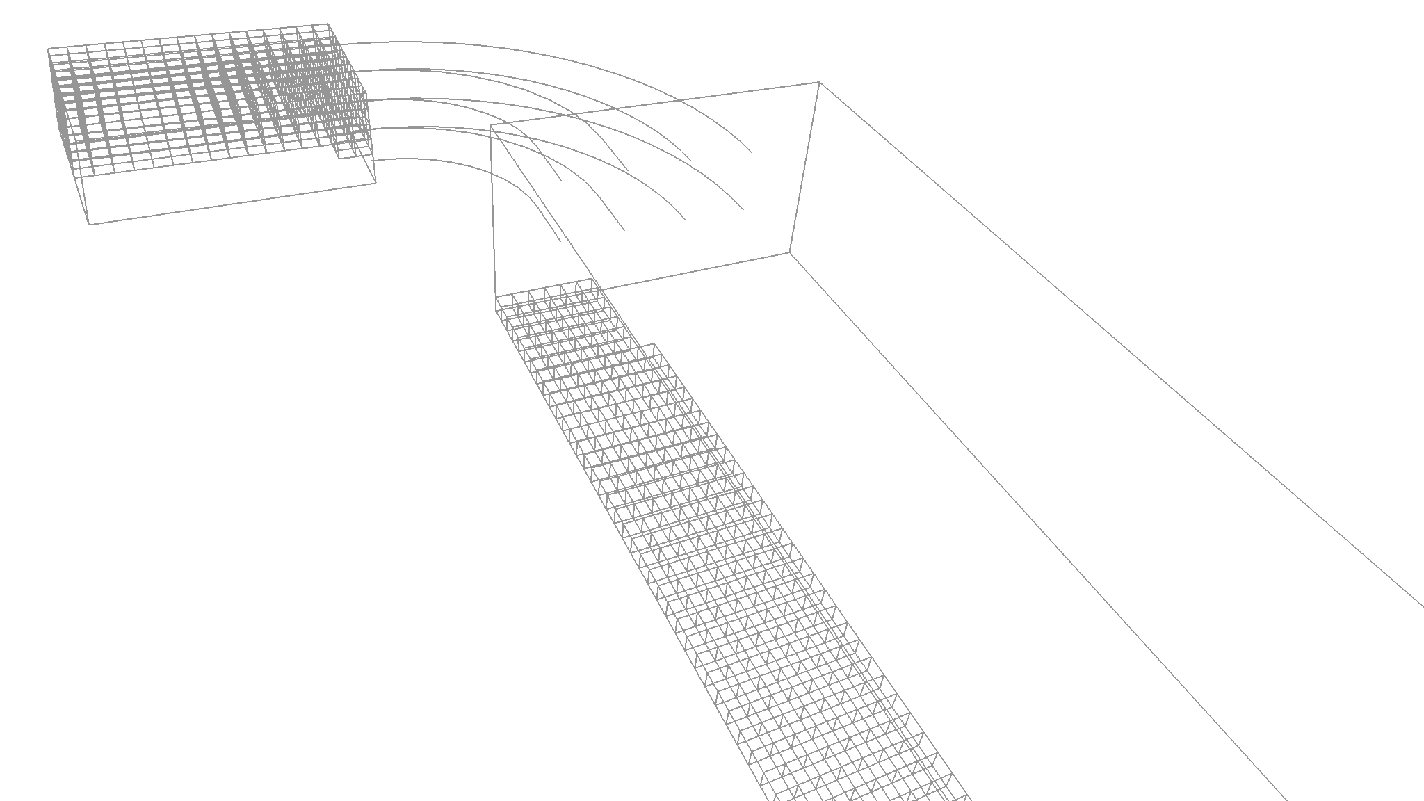
Workflow geo-grid illustrates how to show a subset of the grid’s cells.
Clip Geometry at a Plane or Basic Shapes
You might want to see the inside of the computational domain, but still retain parts of the outer surface. In order to do so, you need to cut the geometry open. Vistle provides two modules for this purpose: the CutGeometry and the ClipVtkm module. They perform similar tasks, but are subject to different limitations.
The CutGeometry module is able to process triangular and polygonal meshes and will ignore any mapped data (e.g. scalar or vector fields) on the geometry.
The ClipVtkm module is able to process unstructured grids and will also clip mapped data. It is not able to work on polygonal (or general polyhedral) meshes. As it is based on the Viskores library, it is able to process large datasets in parallel.
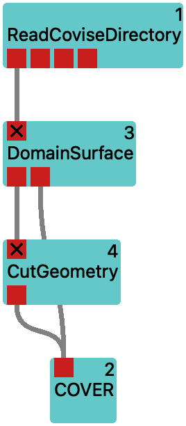
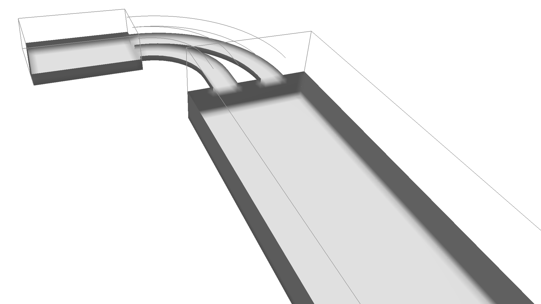
We build on the workflow from the previous section. We want to show a bit of the outer shell of the domain, but also get a view inside. So we add the add the CutGeometry module and connect its input to the first output of DomainSurface and its output to COVER. You can adjust the location of the clip by switching to the COVER window and enabling the Pick interactor in the Vistle -> CutGeometry_? menu. This will bring up a 3D manipulator in the COVER window. Drag with the mouse on the sphere to move the plane and change its orientation by moving the tip of the arrow. When satisfied, disable it again by deselecting the Pick interactor in the menu.
We also want to show cell structure within a spherical subset of the domain.
To do so, we add the ClipVtkm module and connect its input to the output of ReadCoviseDirectory and its output to the input of the existing ShowGrid module.
This will cut the direct connection between ReadCoviseDirectory and ShowGrid.
Make sure to enable visualization of all grid cells supplied to ShowGrid by changing its cells parameter to all.
Now continue to adjust the location of the clip by switching to the COVER window and enabling the Pick interactor in the Vistle -> ClipVtkm_? menu.
Also use this menu in order to change the Surface style from Plane to Sphere.
Also check the Invert menu entry to show the inside of the sphere.
You can adjust the sphere location by moving the sphere manipulator with the cross hairs in the COVER window and its radius by dragging the other sphere manipulator.
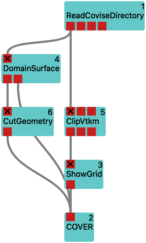
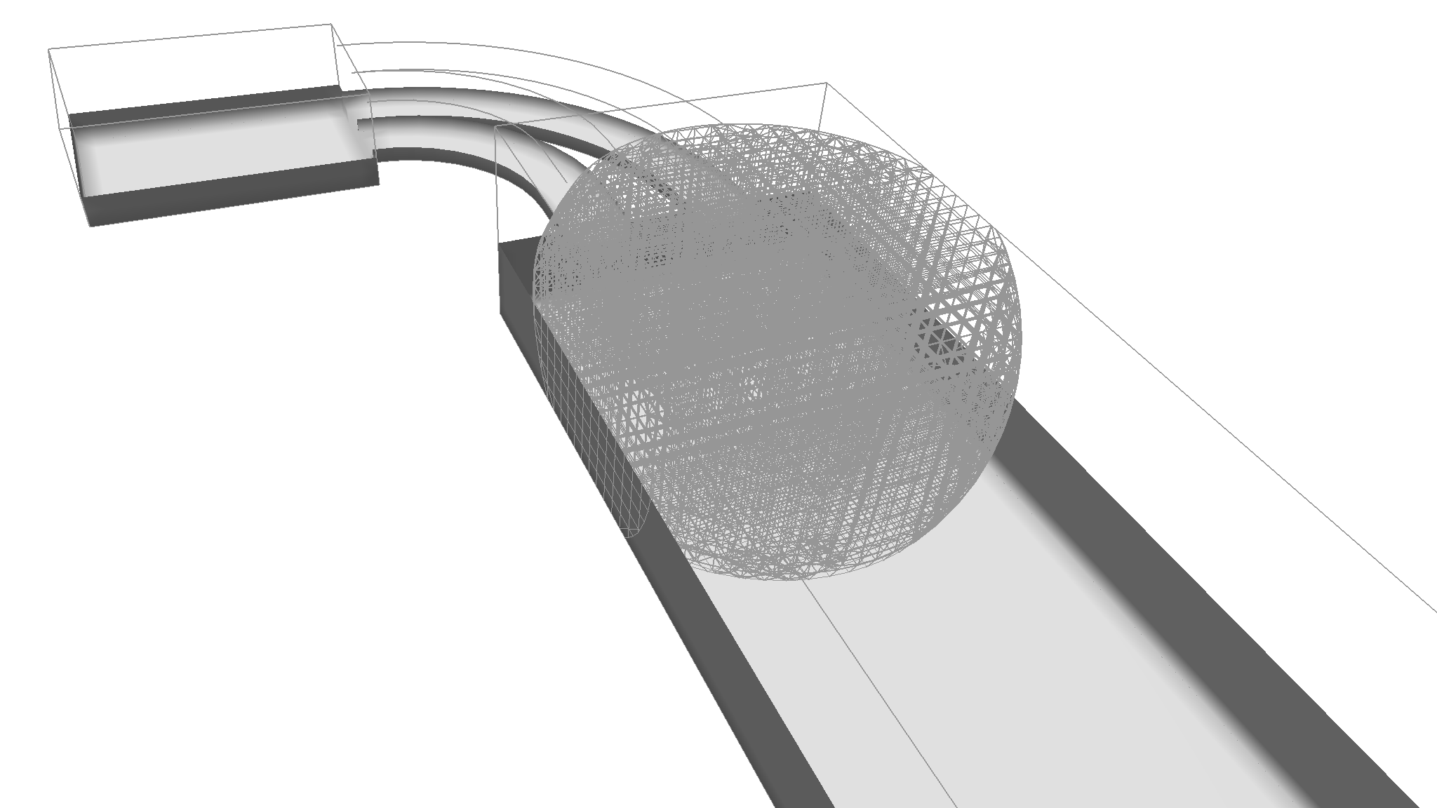
Workflow geo-cut illustrates the results of the geometry clipping operations.
Visualizing Scalar Fields
Up to now, we have only looked at the geometry input for the simulation. Let’s continue with the scalar fields.
Read in an Additional Scalar Field
In order to visualize the scalar fields, we need to read them in first.
We continue where we left off in the previous section.
We remove the the ClipVtkm branch from the workflow by selecting both the ClipVtkm and ShowGrid modules.
From the context menu on either of the selected modules, invoke Delete Selected.
Then we configure the ReadCoviseDirectory module to also read in the pressure field:
select the ReadCoviseDirectory module and select tiny_p from the list of available fields in the field0 parameter.
Workflow press-read adds reading the pressure field.
Explore Scalar Fields via Level Sets with the IsoSurface Module
The IsoSurface module can be used to extract level sets from the scalar fields.
It will create a surface mesh that represents the points in the scalar field where a given value is found.
This technique is often used to visualize the shape of a scalar field.
We are going to apply it to the pressure field.
Add an IsoSurface module to the workflow and connect its first input to the second output (providing the pressure field) of ReadCoviseDirectory.
Then connect its output to the input of COVER.
Executing the workflow will show the surface of the pressure field in the COVER window.
You can adjust the isovalue by selecting the IsoSurface module and changing the isovalue parameter in its parameter window.
You can also use the slider in the Vistle -> IsoSurface_? menu to adjust the isovalue interactively.
Another way to adjust the isovalue is to enable the Pick interactor from this menu: now you can drag the sphere to choose a point that provides the isovalue.
For now, this isosurface will always be shown in a light gray color.

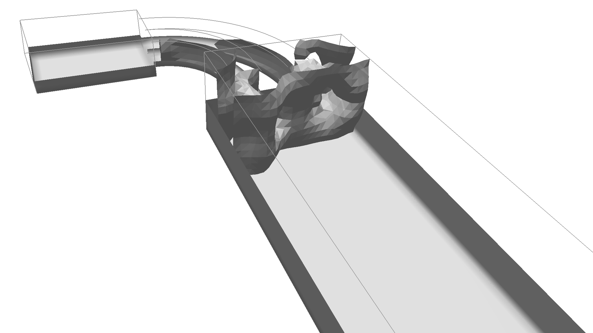
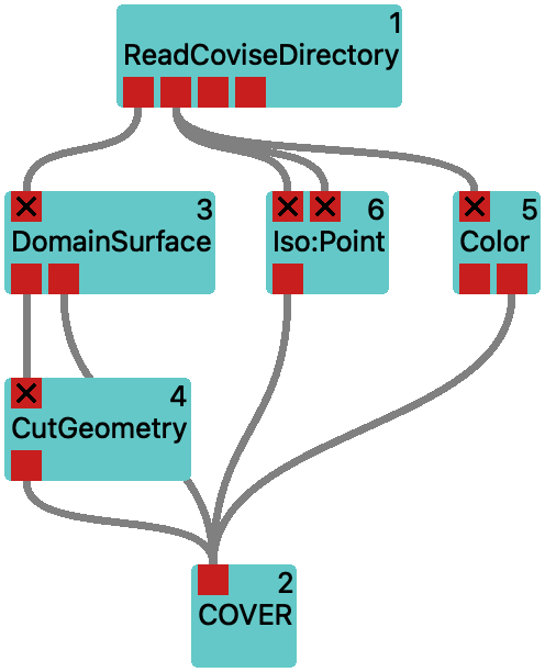
Workflow press-iso explores the pressure field via level sets.
Provide a Color Mapping/Transfer Function for the Scalar Field
Then add a Color module to the workflow and connect its input to the second output of ReadCoviseDirectory.
This forwards the pressure field to the Color module, so that it can detect its minimum and maximum values.
This will be used to provide a color mapping (i.e. transfer function) for the pressure field on its second output.
Connect this to the COVER renderer.
Now, the Vistle -> Color menu in the COVER window will have an entry for this color map.
You can interact with the color map either via this Color_? sub-menu or via the Color module’s parameter dialog in the user interface.
You can make display a color legend by checking the Show entry in the Color_? sub-menu.
You will notice that this Color module carries the label tiny_p.
This means that this color map is used for all subsequent modules that are connected to the second output of ReadCoviseDirectory.
Let’s revisit our isosurface. What about coloring it according to the pressure field so that its color changes whenever we change the value? For that purpose, the IsoSurface module provides a second input t˙hat provides a scalar field to map onto the isosurface. So we connect the second output of ReadCoviseDirectory another time to IsoSurface, but now to its second input. You could use the Pick interactor to adjust the isovalue interactively…
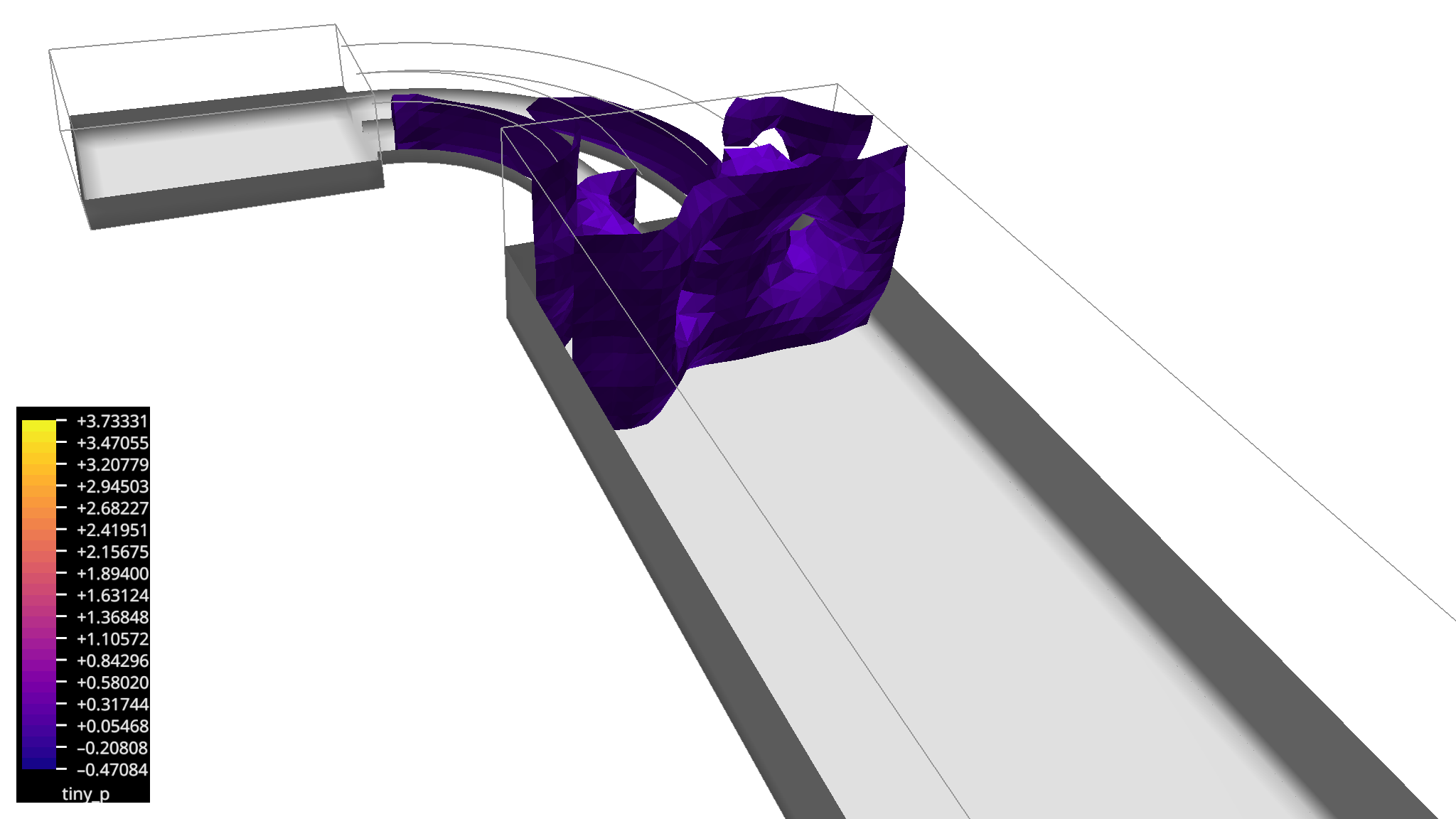
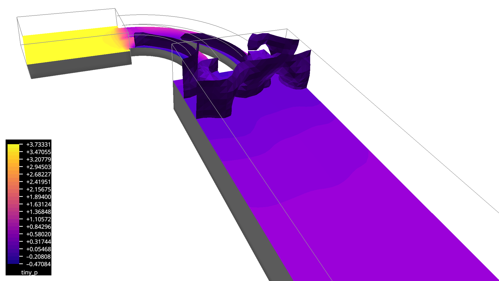
Workflow press-color explores the pressure field via level sets.
Slice a Scalar Field with CuttingSurface
We finish exploring the pressure field by slicing it with the CuttingSurface module.
Add a CuttingSurface module to the workflow and connect its input to the second output of ReadCoviseDirectory.
Then connect its output to the input of COVER.
Execute the workflow and you will see a plane slicing through the pressure field.
You can adjust the position of the plane by selecting the CuttingSurface module and changing the point (a point on the plane) and vertex parameters in its parameter window.
Or you can use the Vistle -> CuttingSurface_? menu in the COVER window to adjust the position of the plane interactively by enabling the corresponding Pick interactor.
Now let’s make use of the color mapping.
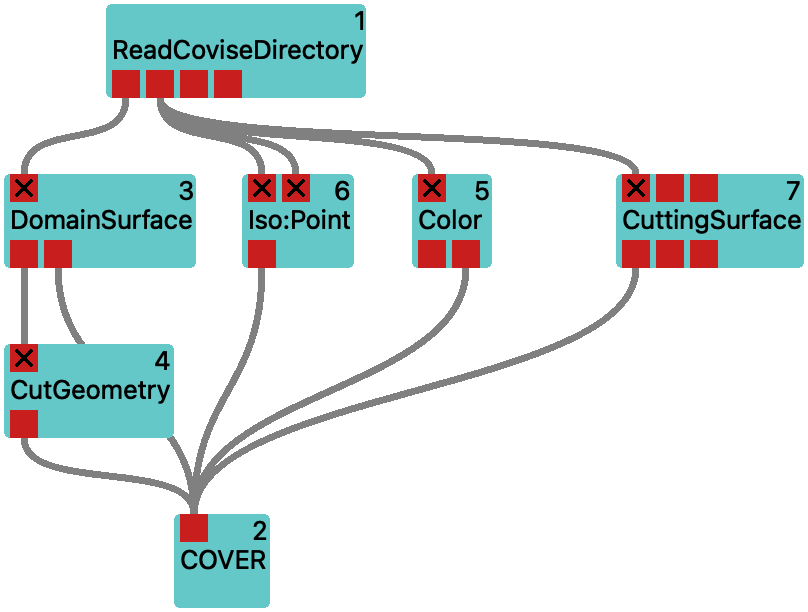
Workflow press-cut shows the pressure field sliced with a plane.